


By: Mayank Anand *, Natasha Hynes, Amit Baroi, Alex Pottier, Kim Davies
Abstract
In the realm of oceanic ecosystems, the vital role of zooplankton in maintaining equilibrium and facilitating essential Earth processes has garnered significant attention. Addressing the intricate challenge of accurately recognizing zooplankton is essential for scientific studies and measurements. However, the manual identification of zooplankton, while indispensable, is hindered by its labor-intensive and time-consuming nature, primarily due to the requirement for specialized expertise. The emergence of deep learning has opened up a transformative avenue for progress, leveraging its impressive performance in various classification and segmentation tasks. In this research, we present an innovative computer vision solution designed to classify shadowgraph images of zooplanktons. Our approach involves an ensemble of convolutional neural networks strategically combined to strike an optimal balance between minimizing False Positives and False Negatives. This concerted fusion has yielded a remarkable inference accuracy of 94.42%. Moreover, we introduce an encoder-decoder Image Segmentation model, enhanced by convolution and deconvolution layers. This model excels in generating masks that surpass the fidelity of true masks, highlighting its potential for meticulous delineation.
1. Introduction
1.1 Motivation
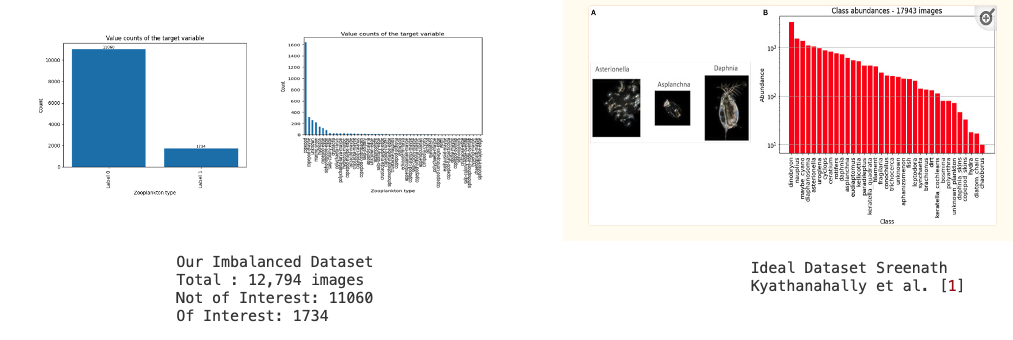
The driving force behind our research originates from the intricate and laborious task of manually identifying zooplankton within shadowgraph images. This process necessitates specialized expertise to discern relevant images, leading to a significant time investment that hinders the progress of concurrent research efforts. Recognizing this predicament as a pivotal concern, we have framed our study to address these challenges and propel the field forward. While considerable research has been conducted in recent times, particularly in lake zooplankton studies such as the work by Sreenath Kyathanahally et al. [1], the challenges are amplified when dealing with seawater from the Bay of Fundy. This environment presents a unique challenge as a substantial portion of the images do not contain identifiable animals. Consequently, this leads to a highly imbalanced dataset, setting it apart from other studies where datasets are more evenly distributed. Convolutional neural networks, although widely successful in balanced datasets, face challenges in our scenario. To highlight the disparity, consider the barplot below, illustrating the distribution of images containing animals in our training dataset in comparison to other freshwater studies.
1.2 Problem Statement
The research focuses on addressing the following problem statement: For a given uncropped image, we aim to determine whether the image contains an animal. Furthermore, if an animal is detected, our objective is to pinpoint its exact location within the image. To address this, we first developed a binary classifier to filter and identify relevant images containing animals. Subsequent to classification, we designed a segmentation model to precisely locate the animal within the selected images.
2. Materials and Methods
2.1 Exploratory Data Analysis and Early Experiments
Our dataset, comprising approximately 41,860 images, offers a wealth of information. Among these, 12,794 images have been meticulously annotated by experts from the Biological Sciences Lab at the University of New Brunswick. Out of these annotated images, 1,734 contain animals. Below, on the left, show the images we obtained after clipping from annotations. We created a small animation from a subset of cropped images, as shown. On the right, we have a similar animation with uncropped images.

The annotations not only identify the presence of animals within the images but also provide precise information about their locations. This information is neatly documented in an accompanying CSV file. It’s worth noting that the annotations vary in form, ranging from polygonal outlines to square bounding boxes, as shown in the images below. These variations posed challenges when creating masks for segmentation later on.

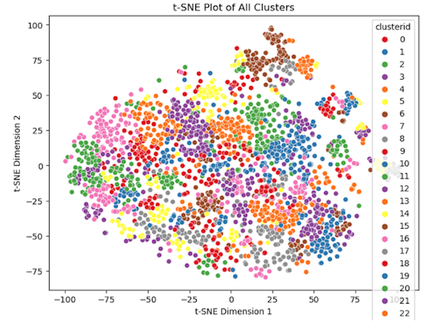
We set out to explore both avenues of deep learning: unsupervised and supervised approaches. We began by employing an unsupervised learning method. We designed two autoencoders to encode two types of images we possessed: uncropped images and cropped images. The latter were generated using annotations from the provided CSV file. Following the encoding process, we applied EM clustering to the resulting latent vectors obtained from encoding these images. Subsequently, we generated t-SNE plots for both experiments. Upon analyzing the clusters, it became apparent that images containing animals displayed a high degree of dispersion, as illustrated in the accompanying t-SNE plots. While we achieved meaningful clusters, the approach faltered for uncropped images due to a significant amount of black pixels present in images from the shadowgraph lens. This led to uninformative latent vectors, resulting in high similarity among most vectors within the vector space.


2.2 Data Preparation and Pre-processing
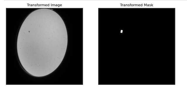
Due to the difficulty of establishing a clear decision boundary between images that were of interest to us and those that were not, we decided to employ supervised learning techniques, specifically deep convolutional neural networks. To ensure compatibility with our models, we standardized the size of all images to 256 x 256. This dimension was chosen through hyperparameter tuning. For the segmentation task, we opted for an image size of 512 x 512. This choice balanced optimal results with the allocated GPU memory, preventing kernel crashes in our AWS Sagemaker Notebooks. We did not apply any transformations for our classification task, but normalized our images with mean = [0.485, 0.456, 0.406], std = [0.229, 0.224, 0.225]. On the other hand, for the segmentation task, data augmentation proved to be invaluable in refining the precision of our decision boundaries when segmenting the animals. Our augmentation strategy encompassed Random Horizontal Flips, Random Vertical Flips, and Random Rotations with variable angles of up to 20 degrees. Furthermore, we substantially augmented our dataset, generating corresponding true masks to enhance the segmentation process.
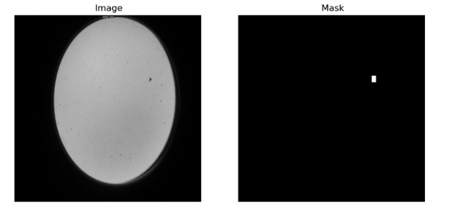
For our segmentation task, it was crucial to have a benchmark or ground truth against which our model’s predictions could be compared. To establish this, we generated true masks, derived from detailed annotations listed in the ‘annotation.csv’ file. These annotations catered to all images that prominently featured animals. This mask creation process is not just a simple binary conversion but involves intricate steps to ensure the masks are accurate and representative of the true distribution and shape of the animals in the images. The image below offers a visual representation, showcasing the meticulous process involved in creating these masks.
2.3 Training, Validation, and Test
To effectively partition our images, we segregated them into distinct training, validation, and test sets. We further reserved a set of 500 images for exclusive use in the testing phase, keeping them entirely separate from the train and validation sets. The remaining images were divided, with 80% designated for the training set and the remaining 20% allocated to the validation set. For the segmentation task, a similar approach was employed. We allocated 80% of the data for the training set, 10% for validation, and the final 10% for testing purposes. In the results section, we present various confusion matrices pertaining to the classification task, specifically focusing on the set of 500 images that were kept aside for the test set. To evaluate the effectiveness of human annotation, we provided the same set of images to human annotators and obtained confusion matrices by comparing our predictions to the actual annotations.
2.4 Deep Learning Architectures
2.4.1 Binary Classification
For binary classification, we designed a convolutional network composed of three convolutional layers, each paired with a ReLU activation function. Following each convolutional layer, we integrated dropout and max-pooling functionalities, together forming a single convolutional block. Our architecture is structured with three such blocks, as illustrated in the subsequent visualization. After the convolutional operations, the design includes three fully connected layers, culminating with a sigmoid function that predicts the likelihood of an image being assigned to the class labeled ‘1’. To bolster the model’s precision, we incorporated a learnable threshold. This threshold, tailored to reduce false negatives, undergoes adjustments after every training epoch, relying on performance metrics from the validation set. The fine-tuned threshold plays a pivotal role in classifying the image. For the optimization process, we employed the Binary Cross-Entropy loss, aiming to minimize its resulting value.

2.4.2 Segmentation
For our segmentation task, we undertook a deliberate analysis and opted to utilize the architecture as presented in the research by Ronneberger et al. [4]. This model has consistently demonstrated superior performance in bioimage segmentation tasks. Given that our images feature distinct, small animals, this U-net architecture was deemed the most appropriate choice.
The model comprises three primary components:
- Encoder Module: This module contains a series of convolutional layers, complemented by MaxPooling operations. Additionally, we incorporated Batch Normalization and Dropout layers within each convolutional block for improved stability and regularization, respectively.
- Bottleneck Layers: Situated between the Encoder and Decoder, this segment consists of a pair of convolutional and deconvolutional layers.
- Decoder Module: The Decoder embodies a sequence of deconvolutional layers, uniquely paired with skip connections from the Encoder. It’s noteworthy to mention that while skip connections are instrumental in our use-case, they aren’t typically integrated into standard autoencoder architectures. Lastly, the model concludes with an output layer comprised of convolutional layers. The output from this layer is then subjected to a Binary Cross Entropy loss, juxtaposed against the true mask. These true masks are generated from annotations provided in an accompanying CSV file. Below, we showcase several sample masks used during the loss computation.

3. Experiments and Results
3.1 Binary Classification
3.1.1 Preliminary Run without Hyperparameter Tuning
In our preliminary run, we employed the ADAM optimizer to minimize the Binary Cross Entropy loss. The learning rate was set to 0.001, and a decay on the learnable parameters was set to 1e-5. This decay acts as an L2 weight decay regularization within our model. We set beta1 to 0.8 and beta2 to 0.999, with an epsilon of 1e-8. Given our dataset’s significant class imbalance, we adjusted the loss function to penalize more heavily when the model incorrectly predicted for the minority class (label ‘1’). This label signifies the presence of an animal in the image. Based on our dataset’s distribution, we determined a penalizing loss ratio: loss_ratio = label_counts[0] / label_counts[1] = [1.0000, 6.3882]. To ensure stability during the initial training phases, we incorporated a learning rate warm-up for the first 100 steps, post which the rate was held constant at 0.001. We trained the model for 30 epochs, and the results, presented in the confusion matrix, are detailed in the following section.
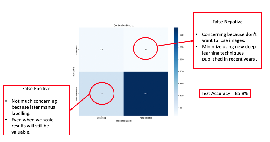
From our early results, we achieved an accuracy of 85.80%. However, we observed a significant number of false positives and false negatives. The primary concern was the false negatives, as losing images in an already imbalanced dataset could be detrimental. Misclassifying and subsequently omitting images could reduce the limited number of images confirming the presence of animals even further. As a result, our subsequent experiments aimed to explore advanced deep learning techniques that could effectively diminish both type I and type II errors in our predictions.
3.1.2 Hyperparameter Tuning using Hyperparameter Grid
We undertook hyperparameter tuning leveraging a hyperparameter grid, focusing on the following parameters:
- Models: Through experimentation with various architectures, it was noted that augmenting the depth of our model precipitated overfitting. This, in turn, affected the model’s validation performance adversely.
- Learning Rate: An array of learning rates (0.1, 0.01, 0.001, and 0.0001) was evaluated. The analysis indicated that a learning rate of 0.001 provided the optimal outcome.
- Weight Decay: We assessed multiple weight decay values, including 1e-3, 1e-4, 1e-5, and 1e-7. The optimal performance was observed with a weight decay of 1e-7.
- Dropout: To counteract overfitting, we experimented with varying dropout rates (0.05, 0.1, 0.2, 0.3, and 0.4). Through these tests, a dropout rate of 0.2 was determined to be the most effective.
- Batch Size: We evaluated the effects of different batch sizes on model performance, specifically sizes of 16, 32, and 64. The batch size of 16 was found to produce the best results.
In our exploration of contemporary deep learning techniques, we incorporated the RAdam Optimizer[2] as proposed by Liu et al. in their research[2]. This replaced our initial choice, the Adam optimizer. Furthermore, we implemented the Lookahead Optimizer technique, setting k to 10, alpha to 0.5, and selecting RAdam[2] as the base optimizer, following the methodology outlined by Zhang et al.[3] in their study. The integration of these techniques substantially improved our results, which are detailed in the subsequent sections.
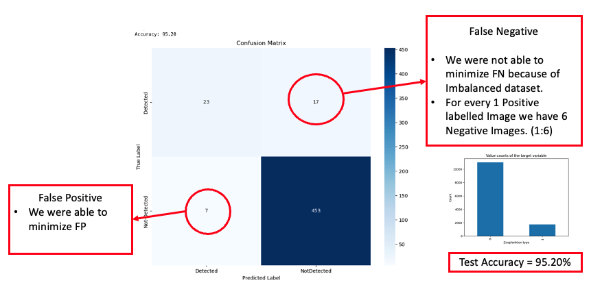
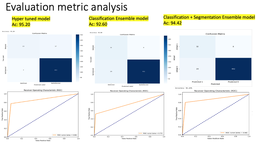
In the visualization presented above, we observed a significant improvement in inference accuracy, reaching 95.20%. While there was a marked reduction in the number of false positives, the presence of false negatives remained a concern.
From the results, it’s evident that the countless hours dedicated to hyperparameter optimization, coupled with the incorporation of recent advancements in the deep learning domain, have yielded improved outcomes. The model’s accuracy surged, achieving a commendable score of 95.20%. While we succeeded in substantially reducing the number of false positives, false negatives continued to pose a significant challenge. Upon analysis, we suspected that the primary reason for this could be the imbalanced nature of our dataset. The model had limited exposure to the minority class, labeled as ‘1,’ which represents images containing animals. This lack of representation is likely a substantial factor behind our inability to effectively minimize false negatives.
3.1.3 Down-Sampling Majority Class
In light of our observations regarding the model’s performance with an imbalanced dataset, we decided to try a different approach. Specifically, we down-sampled our majority class, labeled ‘0’, representing images without animals. By doing so, our goal was to match the count of these images with that of the minority class, labeled ‘1’, indicating the presence of animals. This adjustment notably reduced the total number of images available for training, subsequently diminishing the overall training steps, as the model now had fewer examples to process. Nevertheless, we opted to retain the hyperparameters from our previous experiment, given their demonstrated effectiveness. The results of this experiment are discussed in the sections that follow.
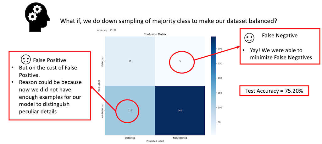
In the visualization presented above, we observed a significant improvement in the reduction of False Negatives after balancing our dataset, but at the cost of the model’s total Accuracy, which decreased to 75.20%.
From our findings, it became clear that down-sampling the dataset effectively addressed the issue of false negatives. However, this came at the expense of the model’s overall accuracy. The drop in accuracy can be attributed to the fact that down-sampling the majority class left us with significantly fewer examples for training, impacting the model’s performance. Additionally, we experimented with up-sampling the minority class by generating new examples of images with animals. This involved applying similar transformations as we did for the segmentation task. However, this strategy didn’t yield the anticipated improvements in our results.
3.1.4 The Ensemble of Models
In our pursuit of finding the ideal balance between minimizing false negatives and false positives without sacrificing the model’s overall accuracy, we devised a novel ensemble approach. This approach combined the strengths of the models we examined in our earlier experiments. The core idea was to amalgamate the high accuracy of one model with the diminished false negatives of the other, achieved by taking a weighted average of their predictions. Importantly, determining the exact weighted average emerged as a new hyperparameter challenge. After multiple iterations, we identified an optimal mix that offered a commendable balance between both type I and type II errors while maintaining the model’s high accuracy. This innovative ensemble method underscores the advantages of merging different models in machine learning. By capitalizing on the distinct strengths of each model, we overcame previous challenges, emphasizing the principle that collaborative approaches often yield superior results in deep learning experiments.
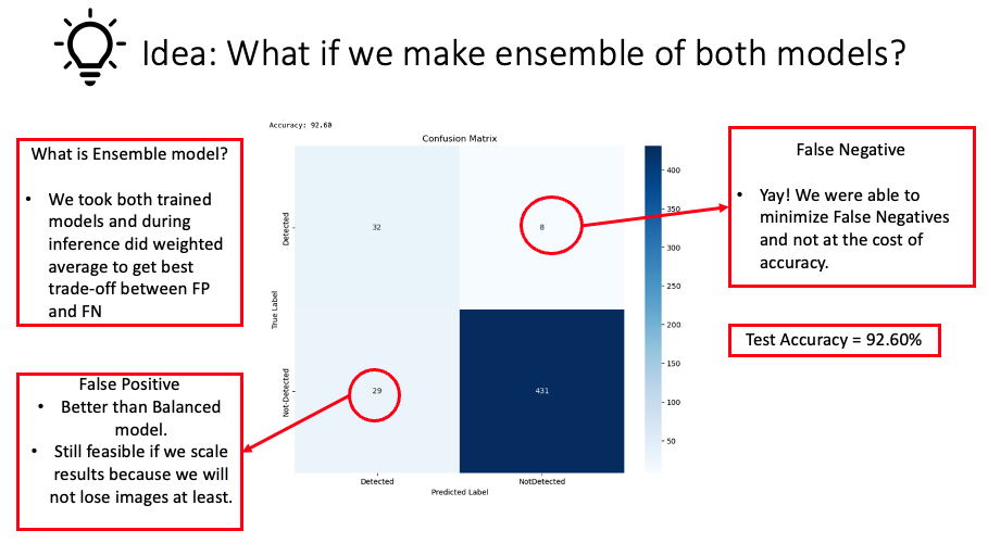
From the visualization provided above, we observed a significant reduction in false negatives after employing an ensemble of the previous two models, with only a minimal impact on accuracy (92.60%).
From the presented confusion matrix, it’s evident that the ensemble method is the optimal approach for this problem. By utilizing this method, we significantly reduced false negatives with only a minimal compromise in accuracy. Moreover, these results not only validate but also emphasize our model’s robust capability in classifying images. The impressive accuracy levels combined with minimized type II errors underscore the model’s reliability and effectiveness. This accomplishment, when seen in the broader perspective, strengthens the case for adopting ensemble methods in similar challenges, reflecting their inherent strength in capitalizing on the best attributes of individual models to produce an enhanced overall result.
3.2 Segmentation
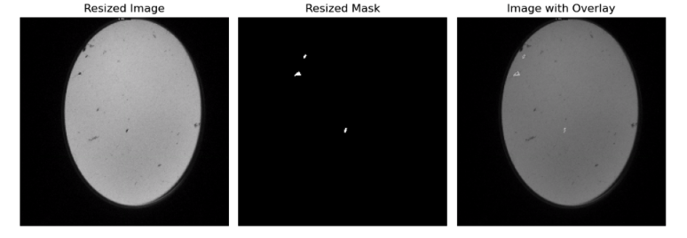
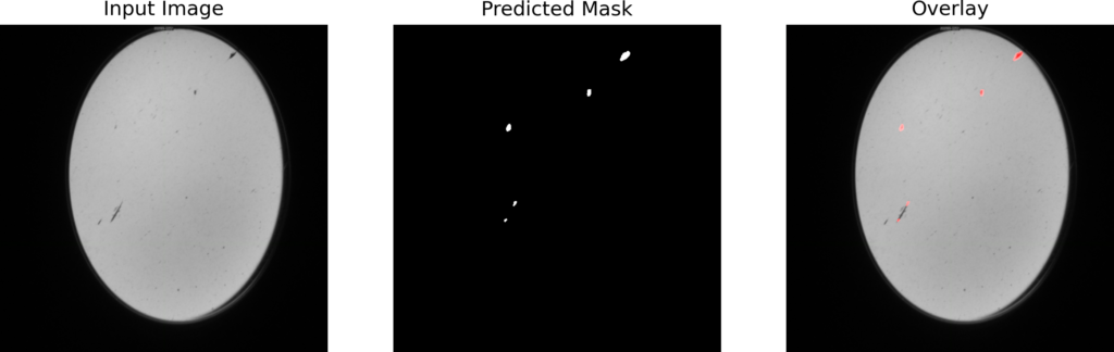
For our segmentation task, we employed the RAdam Optimizer [2] with a learning rate of 0.001 to optimize the Binary Cross Entropy loss. The model was trained over 100 epochs. As demonstrated in the images below, the masks obtained on the validation set surpassed the quality of the true masks. Notably, our model could detect and segment multiple animals within a single image.
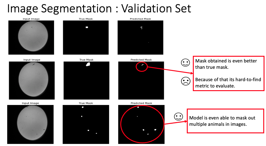
This image displays the output masks produced by our model on the validation set. As seen, the quality and precision of the segmentation surpass that of the true masks. Multiple animals within the image are distinctly segmented, highlighting the model’s proficiency.
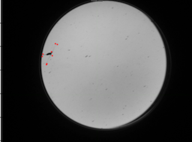
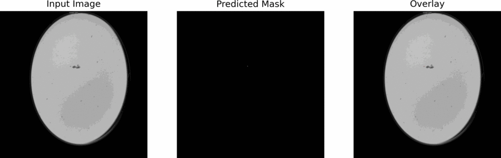
It’s interesting to note that in our annotations, there were a few instances where even our human annotators couldn’t confidently determine the presence of animals in certain images. However, when we examined the results from our model, we were quite impressed. The model managed to identify animals in those challenging pictures, where even our eyes had doubts, as shown in the image below with the image name highlighted in red.
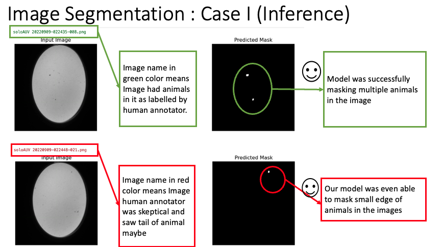
Here, we have a challenging image where even our human annotators were on the fence about the presence of animals. Remarkably, our model rose to the challenge, confidently identifying and segmenting potential animals in these areas of ambiguity.
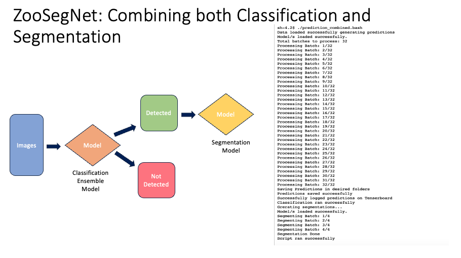
3.3 ZooSegNet: Combining both Classification and Segmentation
We introduced ZooSegNet, a seamless integration of both classification and segmentation models. The primary objective of this approach was to first discern images that contain animals, and subsequently, to precisely locate these animals within the detected images.
3.3.1 Methodology
Upon receiving the input images, a Python script was employed. This script first classified the images, moving them to either ‘Detected’ or ‘NotDetected’ folders based on their content. Following classification, the segmentation model was applied solely to the images in the ‘Detected’ folder.
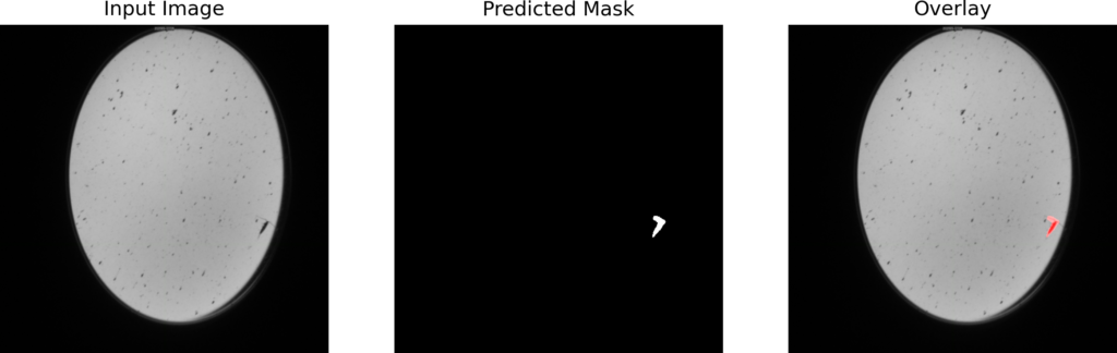
3.3.2 Qualitative Results
Single Animal Segmentation: The leftmost image showcases our model’s ability to accurately segment a lone animal. The overlaid mask highlights the exact location of the animal in the original image.
Multiple Animal Segmentation: The next image to the right demonstrates how our model effectively handles scenes with several animals, ensuring each one is clearly segmented without missing any.
3.3.3 Quantitative Results
In a deeper exploration of our test set, an intriguing trend emerged. Certain images that misled our classification model did not deceive our segmentation model. Interestingly, the masks produced for these specific images were predominantly black. Further investigation revealed that these images corresponded to the false positives overlooked by our classification model. This finding highlights the efficacy of our ensemble technique, “ZooSegNet”. By combining both models, the ensemble enhances the network’s reliability, bolstering it against potential misclassifications. The effectiveness of ZooSegNet is demonstrated by its impressive performance metrics. Notably, our ensemble outperformed the standalone classification model, boosting accuracy by 2% to achieve an outstanding 94.42% on the inference dataset. Subsequent sections will compare the evaluative measures and illustrate the results using the associated ROC curve, emphasizing the improved performance and reliability of our combined strategy.
This animated GIF comprises a sequence of nine images, illustrating the areas where our ZooSegNet ensemble demonstrated remarkable precision. Each image presents black masks, emphasizing instances where the classification model misjudged, but the segmentation approach astutely rectified these inaccuracies. These visual results underscore the ensemble’s strength in providing a more comprehensive detection framework, successfully pinpointing and adjusting for the classification model’s occasional oversights.
4. Source Code and Reproducibility
Our Python script and source code are available on GitHub at the following link. Click here.
5. Conclusion
Exploring the vast depth of ocean data, especially the enigmatic zooplankton, was always a formidable task. It demanded intense dedication, specific knowledge, and considerable time. Nevertheless, this research highlighted the powerful role of deep learning as an ally in this exploration. While our early attempts faced hurdles like false negatives and the issues presented by imbalanced datasets, determination is a foundational principle in science. By continuously innovating, we not only minimized these errors but also created a groundbreaking ensemble technique that combined the advantages of multiple models. This effort yielded an impressive accuracy of 94.42%.
However, the real success is not just in the statistics. The genuine accomplishment is the practical impact of our work. The once daunting process of categorizing and pinpointing zooplankton in shadowgraph images is now substantially more efficient. Moreover, our system, ZooSegNet, with its dual role in classification and segmentation, demonstrates the potential of combined methods in addressing the shortcomings of standalone models. To wrap up, reflecting on our journey underscores that the significance of this research extends beyond its direct outcomes. It highlights the value of tenacity, teamwork, and creativity in the realm of science. The vast and mysterious ocean remains a challenge for many, but with innovations like ours, we edge closer to unveiling its secrets.
6. Acknowledgements
The shadowgraph camera was developed by Williamson and Associates Technologies (Seattle, WA) and loaned from Christian Reiss at the NOAA Southwest Fisheries Science Centre for the project. The images were collected with funding and logistical support from the Ocean Tracking Network, Tides Foundation, Fisheries and Oceans Canada – Canada Nature Fund for Aquatic Species at Risk, and the Canadian Wildlife Federation. The research was a collaboration between DeepSense and the Davies Lab at the University of New Brunswick. Natasha Hynes and Emma Chaumont in the Davies Lab annotated the imagery for the project.
7. References
Kyathanahally, S. P., Hardeman, T., Merz, E., Bulas, T., Reyes, M., Isles, P. D. F., Pomati, F., & Baity‐Jesi, M. (2021b). Deep learning classification of Lake Zooplankton. Frontiers in Microbiology, 12. https://doi.org/10.3389/fmicb.2021.746297
Liu, L. (2020, April 1). On the Variance of the Adaptive Learning Rate and Beyond. https://iclr.cc/virtual_2020/poster_rkgz2aEKDr.html
Ronneberger, O., Fischer, P., & Brox, T. (2015). U-NET: Convolutional Networks for Biomedical Image Segmentation. In Lecture Notes in Computer Science (pp. 234–241). https://doi.org/10.1007/978-3-319-24574-4_28
Zhang, M. R., Lucas, J., Hinton, G., & Ba, J. (n.d.). Lookahead optimizer: K steps forward, 1 step back. Department of Computer Science, University of Toronto, Vector Institute. https://www.cs.toronto.edu/~hinton/absps/lookahead.pdf